StatsNotebook

Descriptive statistics

20 Sep, 2020 | 6 minutes read

Tags: Analysis, R code, Descriptive statistics

Follow our Facebook page or our developer’s Twitter for more tutorials and future updates.

The tutorial is based on R and StatsNotebook, a graphical interface for R.

This tutorial will give a short introduction on descriptive analysis using StatsNotebook. Descriptive statistics such as mean, standard deviation, median and interquartile range can be easily obtained using the Explore panel.

We use the built-in Personality dataset in this example. This dataset can be loaded into StatsNotebook using the instructions provided here or can be downloaded from here .

This dataset can also be loaded using the following codes

library(tidyverse)
currentDataset <- read_csv("https://statsnotebook.io/blog/data_management/example_data/personality.csv")

The Personality dataset contains data from 231 participants, with measures on the Big 5 personality factors (Agreeableness, Conscientiousness, Extraversion, Neuroticism and Openness), and three measures of mental health (Depression, Trait anxiety and State anxiety). It also contains data on participants’ sex.

We will demonstrate how to generate simple descriptive statistics, and how to generate descriptive statistics by group.

Descriptive statistics

To calculate descriptive statistics,

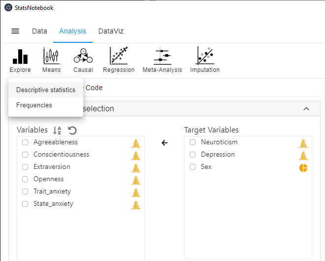
Click Analysis at the top
Click Explore
Select Descriptive statistics on the menu
Select variables into Target Variables on the right. In this example, we will select Neuroticism, Depression and Sex.
- Sex is a categorical variable. If it is not yet coded as a factor, we will need to manually convert it into a factor variable.

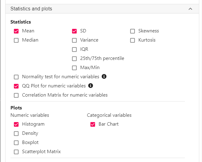
Expand the Statistics and plots panel, by default, mean and standard deviation are calculated for a numeric variable (Neuroticism and Depression); count is calculated for a categorical (factor) variable (Sex). Additional statistics, such as median and interquartile range can be requested here.

R codes - Descriptive statistics

The following is the R code generated by StatsNotebook. We will explain these codes in the next section.

library(tidyverse)
library(e1071)
library(ggplot2)
library(GGally)

"Sample size and missing data"

currentDataset %>%
  summarize(count = n(), 
  mis_Neuroticism = sum(is.na(Neuroticism)), 
  mis_Depression = sum(is.na(Depression)), 
  mis_Sex = sum(is.na(Sex))
  )

"Descriptive Statistics for numeric variables"

currentDataset %>%
  summarize(count = n(),
  M_Neuroticism = mean(Neuroticism, na.rm = TRUE),
  M_Depression = mean(Depression, na.rm = TRUE),
  SD_Neuroticism = sd(Neuroticism, na.rm = TRUE),
  SD_Depression = sd(Depression, na.rm = TRUE)
  ) %>% 
  print(width = 1000, n = 500)

ggplot(currentDataset) +
  geom_qq(aes(sample=Neuroticism))

ggplot(currentDataset) +
  geom_qq(aes(sample=Depression))

ggplot(currentDataset) +
  geom_histogram(aes(x=Neuroticism), color = "white")

ggplot(currentDataset) +
  geom_histogram(aes(x=Depression), color = "white")


"Counts for categorical variables"

currentDataset %>%
  drop_na(Sex) %>%
  group_by(Sex) %>%
  summarize(count = n()) %>% 
  spread(key = Sex, value = count)


ggplot(currentDataset) +
  geom_bar(stat = "count", aes(x=Sex))

"Chan, G. and StatsNotebook Team (2020). StatsNotebook. (Version 0.1.0) [Computer Software]. Retrieved from https://www.statsnotebook.io"
"R Core Team (2020). The R Project for Statistical Computing. [Computer software]. Retrieved from https://r-project.org"

R codes explained - Descriptive statistics

The following is from the top section of the generated codes.

library(tidyverse)
library(e1071)
library(ggplot2)
library(GGally)

"Sample size and missing data"

currentDataset %>%
  summarize(count = n(), 
  mis_Neuroticism = sum(is.na(Neuroticism)), 
  mis_Depression = sum(is.na(Depression)), 
  mis_Sex = sum(is.na(Sex))
  )

First we load all the necessary libraries for this analysis, and then calculate the sample size and missing data in each of the variables. The above codes produce the summary below. Overall, there are 231 rows of data (N = 231). There are 14 missing data points for Neuroticism and 33 missing data points for Depression. There is no missing data for Sex.

######################################################
[1] "Sample size and missing data"

######################################################
# A tibble: 1 x 4
  count mis_Neuroticism mis_Depression mis_Sex
  <int>           <int>          <int>   <int>
1   231              14             33       0


######################################################

The following code is then used to calculate the descriptive statistics for the numeric variables (Neuroticism and Depression).

print("Descriptive Statistics")

"Descriptive Statistics for numeric variables"

currentDataset %>%
  summarize(count = n(),
  M_Neuroticism = mean(Neuroticism, na.rm = TRUE),
  M_Depression = mean(Depression, na.rm = TRUE),
  SD_Neuroticism = sd(Neuroticism, na.rm = TRUE),
  SD_Depression = sd(Depression, na.rm = TRUE)
  ) %>% 
  print(width = 1000, n = 500)

This code produces the following output. The mean of Neuroticism and Depression are 87.7 (SD = 7.06) and 23.1 (SD = 5.81) respectively.

######################################################
[1] "Descriptive Statistics for numeric variables"

######################################################
# A tibble: 1 x 5
  count M_Neuroticism M_Depression SD_Neuroticism SD_Depression
  <int>         <dbl>        <dbl>          <dbl>         <dbl>
1   231          87.7         7.06           23.1          5.81

######################################################

The following code is then used to produce normality plots and histograms.

ggplot(currentDataset) +
  geom_qq(aes(sample=Neuroticism))

ggplot(currentDataset) +
  geom_qq(aes(sample=Depression))

ggplot(currentDataset) +
  geom_histogram(aes(x=Neuroticism), color = "white")

ggplot(currentDataset) +
  geom_histogram(aes(x=Depression), color = "white")

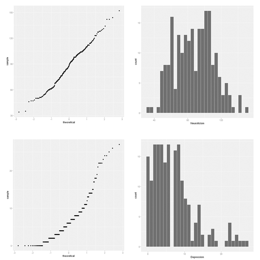
The top two plots are for Neuroticism and the bottom two for Depression. The left plots are normality plots. If the data is normally distributed, the points will roughly follow a straight line. The histograms on the right show the distribution of the variables. These plots show that the distribution of Neuroticism is approximately normal, but Depression is skewed to the right.

Lastly, the following codes are used to calculate the frequency count for the categorical variable Sex and to generate a simple bar graph.

"Counts for categorical variables"

currentDataset %>%
  drop_na(Sex) %>%
  group_by(Sex) %>%
  summarize(count = n()) %>% 
  spread(key = Sex, value = count)


ggplot(currentDataset) +
  geom_bar(stat = "count", aes(x=Sex))

Below is the output from StatsNotebook. Of the 231 participants, 70 are female and 161 are male.

# A tibble: 1 x 2
  Female  Male
   <int> <int>
1     70   161

Descriptive statistics by group

In this example, we will generate the descriptive statistics of Neuroticism and Depression by Sex.

To do this, we can

Click Analysis at the top
Click Explore
Select Descriptive statistics on the menu
Select variables into Target Variables on the right. In this example, we will select Neuroticism and Depression.
Select the grouping variable (Sex) into Split by box on the right.
- Sex is a categorical variable. If it is not yet coded as factor, we will need to manually convert it into a factor variable.
Expand the Statistics and plots panel, by default, mean and standard deviation are calculated for numeric variables (Neuroticism and Depression). Additional statistics, such as median and interquartile range can be requested here.

R codes - Descriptive statistics by group

This code is very similar to those above, except now we have specified that the analysis split by group (Sex).

library(tidyverse)
library(e1071)
library(ggplot2)
library(GGally)

"Sample size and missing data"

currentDataset %>%
  summarize(count = n(), 
  mis_Neuroticism = sum(is.na(Neuroticism)), 
  mis_Depression = sum(is.na(Depression)), 
  mis_Sex = sum(is.na(Sex))
  )

"Descriptive Statistics for numeric variables"

currentDataset %>%
  group_by(Sex) %>%
  summarize(count = n(),
  M_Neuroticism = mean(Neuroticism, na.rm = TRUE),
  M_Depression = mean(Depression, na.rm = TRUE),
  SD_Neuroticism = sd(Neuroticism, na.rm = TRUE),
  SD_Depression = sd(Depression, na.rm = TRUE)
  ) %>% 
  print(width = 1000, n = 500)

ggplot(currentDataset) +
  geom_qq(aes(sample=Neuroticism)) +
  facet_wrap(~Sex)

ggplot(currentDataset) +
  geom_qq(aes(sample=Depression)) +
  facet_wrap(~Sex)

ggplot(currentDataset) +
  geom_histogram(aes(x=Neuroticism), color = "white") +
  facet_wrap(~Sex)

ggplot(currentDataset) +
  geom_histogram(aes(x=Depression), color = "white") +
  facet_wrap(~Sex)

"Chan, G. and StatsNotebook Team (2020). StatsNotebook. (Version 0.1.0) [Computer Software]. Retrieved from https://www.statsnotebook.io"
"R Core Team (2020). The R Project for Statistical Computing. [Computer software]. Retrieved from https://r-project.org"

The output from StatsNotebook are very similar to what we have before but is now stratified by Sex.

######################################################
# A tibble: 2 x 6
  Sex    count M_Neuroticism M_Depression SD_Neuroticism SD_Depression
  <fct>  <int>         <dbl>        <dbl>          <dbl>         <dbl>
1 Female    70          96.2         8.74           23.0          5.87
2 Male     161          83.8         6.16           22.2          5.60

######################################################

Follow our Facebook page or our developer’s Twitter for more tutorials and future updates.