StatsNotebook

The tutorial is based on R and StatsNotebook, a graphical interface for R.

In multiwave longitudinal study, the exposure is often time-varying. A time varying confounder is a time varying variable that is affected by previous exposures, and also affect future exposure and outcome, thus confounding the relationship between the exposure and the outcome. Time varying confounding is common in longitudinal research. When evaluating the relationship between a time-varying exposure and outcome, standard methods such as regression and generalised linear models produce biased estimates in the presence of time-varying confounders. Inverse probability treatment weight and marginal structural model can be used to adjust for time-varying confounding.

In this tutorial, we will use a simulated dataset to answer the following research question

• Does cannabis use during adolescence cause illicit drug use in adulthood?

The example data can be downloaded from here . In this example, we will use a complete dataset (i.e. no missing data). If your dataet has missing data, we would recommend that you read this tutorial and then our tutorial on inverse probability treatment weighting with missing data.

Supposed that the data was collected over 5 time points, baseline (wave 0) and follow-up wave 1 to 4. The baseline and wave 1 to 3 were collected at Grade 7, 8, 9 and 10. Wave 4 was collected at age 25.

In this dataset, there are several key variables.

1. Academic grade (failed; 0: no failed subjects; failed at least one subject)
2. Peers’ cannabis use (peer_can: 0: None; 1: 1-2 friends used cannabis; 2: 3 or more friends used cannabis)
3. Antisocial behaviour (antisocial: 0: No antisocial behaviour; 1: engaged in antisocial behaviour)
4. Cannabis use (can; 0: No use; 1: used)
5. Sex (sex; 0: male; 1: female)
6. Family history of drug use (family_drug_use; 0: no; 1: at least one immediate family member used drug. This is only measured at baseline.)
7. Illicit drug use at age 25 (illicit: 0: No use; 1: used)

The suffix of each variable indicates the time point the data is collected. For example, peer_can_0 represent the number of peers who used cannabis at baseline (wave 0).

This dataset can also be loaded using the following codes

library(tidyverse)
currentDataset <- read_csv("https://statsnotebook.io/blog/data_management/example_data/iptw_example.csv")

Given this design, we can now make our research question more specific

• Does cannabis use in follow-up wave 1 to wave 3 (in Grade 8, 9 and 10) cause use of illicit drug at age 25?

In this research question, cannabis use is the exposure variable and is time-varying. When estimating the relationship between adolescent cannabis use (wave 1 to wave 3) on future illicit drug use, many of the variables above are likely to be time-varying confounders. The figure below is a conceptual diagram demonstrating the complex relationships between the exposure, confounders and the outcome.

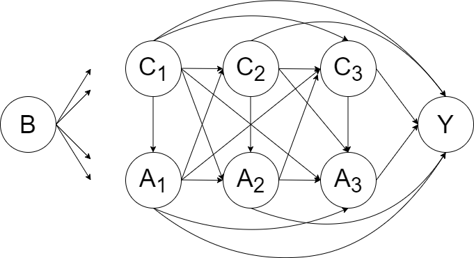
B represents a set of baseline covariates/ potential confounders (e.g. family history of drug use). It can be regarded as a special subset of C₁.
A₁, A₂ and A₃ represent the exposures (cannabis use) at Wave 1, 2 and 3.
C₁, C₂ and C₃ represent the set of covariates/confounders for the exposure variable at Wave 1, 2 and 3 (e.g. peers’ cannabis use). To retain the temporal order of exposure and confounders, the set C₁, C₂ and C₃ should be selected from the preceding wave of the exposure. Therefore, the variables in the set C₁, C₂ and C₃ should be from baseline, follow-up wave 1 and follow-up wave 2 respectively.

Y is the outcome (illicit drug use at age 25).

Take Peers’ cannabis use as an example. Peers’ cannabis use is likely to be a time-varying confounder because

1. An individual’s cannabis use in one wave is likely to increase affiliation with cannabis using peers in future waves.
2. Peers’ cannabis use in one wave is likely to increase the risk of an individual’s cannabis use and illicit drug use in future waves

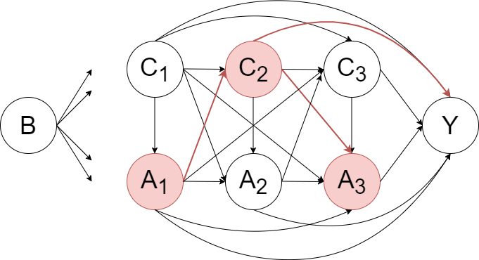
Therefore, peers’ cannabis use is a time-varying mediator (because it was affected by previous cannabis use and would affect future illicit drug use) and a time-varying confounder (because it would affect both future cannabis use and future illicit drug use). Other variables, such as antisocial behaviour, are also likely to be time-varying confounders.

Regression-based methods generally give biased estimates of the effects of time-varying exposures on an outcome when time-varying confounders are present. In the example above, adjusting for peers’ cannabis use at wave 2 will block some of the effect of cannabis use at wave 1. Not adjusting for peers’ cannabis use at wave 2 will bias the estimate of cannabis use at wave 3 on future illicit drug use. This is because peers’ cannabis use at wave 2 may confound the relationship between cannabis use at wave 3 and illicit drug use at the final wave. Therefore, performing a regression analysis would produce biased estimate, regardless of whether adjustment is made for peers’ cannabis use.

Inverse probability treatment weighting (IPTW) can be used to estimate the causal effect of cannabis use on future illicit drug use. Conceptually, IPTW attempts to fully adjust for measured confounders by balancing the confounders across levels of treatment with treatment weight. It creates a pseudo-population in which all measured confounders are balanced between different treatment groups (in the example above, it will be between different cannabis use trajectories). The data can be regarded as coming from a randomized controlled trial and thus causal inference can be made by simple comparisons between groups (i.e. t-test).

For valid causal inference, the following key assumptions need to be met.

1. Exchangeability

   • This is also known as the no unmeasured confounding assumption. It is assumed that all confounders are used to calculate IPTW. While it is nearly impossible to include all confounders in the IPTW calculation, we will need to select a wide range of potential confounders based on a theoretical framework to improve the validity of this assumption. In our example, we determine that family, peer and school variables are important confounders that could affect both adolescent cannabis use and future illicit drug use. We therefore include family history of drug use, peers’ cannabis use, academic grade and antisocial behaviour to calculate IPTW.

2. Positivity

   • The probability of receiving treatment (i.e. using cannabis in our example) and not receiving treatment are both non-zero. This assumption is violated if treatment is deterministic. (e.g. if all children of parents who have used illicit drugs will later use cannabis, this assumption is violated.)

3. Correctness of the model for calculating the IPTW

   • Logistic regressions are usually used to estimate IPTW. Interaction terms can be included into the model to improve the validity of this assumption. Machine learning models can also be used to calculate IPTW to capture potential non-linear effect.

Now we will demonstrate using the simulated example data to test the cumulative exposure effect of cannabis use from follow-up wave 1 to wave 3 on future illicit drug use at wave 4. We will provide a step-by-step guide on how to use StatsNotebook to generate the R codes to calculate IPTW. Then we will conduct a weighted analysis on the weighted sample. The ipw package will be used to calculate the IPTW, and the survey package will be used to conduct the weighted analysis.

We will first calculate the weight at each time point by calculating the probability of receiving/ not receiving treatment, based on the treatment history from previous waves, the history of confounders and baseline confounders/ covariates. In our example, we will need to calculate the weight at follow-up wave 1 to 3 separately, and then calulate a final IPTW by multiplying the three weights from follow-up wave 1 to 3.

1. To calculate the weight at follow-up wave 1, we use the variables from C₁, including academic grade, peers’ cannabis, antisocial behaviour, cannabis use, sex and family history of drug use at baseline.
2. To calculate the weight at follow-up wave 2, we use all the variables from the previous step, plus academic grade, peers’ cannabis and antisocial behaviour at follow-up wave 1 (history of all confounders), and cannabis use at follow-up wave 1 (exposure history).
3. To calculate the weight at follow-up wave 3, we use all the variables from the previous step, plus academic grade, peers’ cannabis and antisocial behaviour at follow-up wave 2, and cannabis use at follow-up wave 2.

Using StatsNotebook - Calculating IPTW

Prior to calculating the IPTW, we will need to conduct a descriptive analysis and it is always good practice to visualise the data.

To calculate the IPTW,

1. Click Analysis at the top
2. Click Causal in the top menu
3. Click Inverse Probability Treatment Weighting (IPTW) in the pop-up menu
4. In the left panel, select can_1 into Exposure, and select failed_0, peer_can_0 and antisocial_0 into Time-varying covariates. As mentioned before, since baseline confounders/covariates can be regarded as a special subset of Time-varying covariates at Wave 1, we further select family_drug_use, sex and can_0 (baseline cannabis use) into Time-varying covariates.
   • To ensure the temporal order of the variables, we use covariates from baseline to calculate IPTW for exopsure at follow-up wave 1.

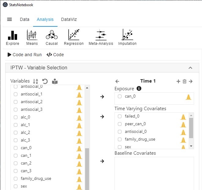
5. Click the top + button on top of Exposure to add an extra time point (extra wave).
6. Select can_2 into Exposure, and select failed_1, peer_can_1 and antisocial_1 into Time-varying covariates.

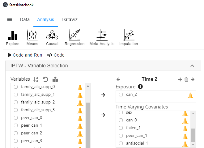
7. Repeat step 5 and 6 for can_3.
8. Expand the panel Analysis Setting at the below the variable selection panel.
9. For Distribution family, select Binomial.
   • Since the exposure is a dichotomised variable (cannabis use or no cannabis use), logistic regression will be used to estimate the IPTW.

10. Click Code and Run. The R codes below will be generated and executed.

Four new variables, .ipw0, .ipw1, .ipw2 and .final_weight will be created. The first three are the IPTW at follow-up wave 1 to 3 and the last one is the product of the first three weights and will be used for subsequent outcome modelling.

R codes - Calculating IPTW

library(ipw)

"Calculate IPTW"

weight <- ipwpoint(exposure = can_1, family = "binomial", link = "logit",
  numerator =~ 1,
  denominator =~ failed_0+peer_can_0+antisocial_0+family_drug_use+sex+can_0,
  trunc = 0.01, data = as.data.frame(currentDataset))
currentDataset$.ipw0 = weight$weights.trunc

weight <- ipwpoint(exposure = can_2, family = "binomial", link = "logit",
  numerator =~ can_1,
  denominator =~ can_1+failed_0+peer_can_0+antisocial_0+family_drug_use+sex+can_0+failed_1+peer_can_1+antisocial_1,
  trunc = 0.01, data = as.data.frame(currentDataset))
currentDataset$.ipw1 = weight$weights.trunc

weight <- ipwpoint(exposure = can_3, family = "binomial", link = "logit",
  numerator =~ can_1+can_2,
  denominator =~ can_1+can_2+failed_0+peer_can_0+antisocial_0+family_drug_use+sex+can_0+failed_1+peer_can_1+antisocial_1+failed_2+peer_can_2+antisocial_2,
  trunc = 0.01, data = as.data.frame(currentDataset))
currentDataset$.ipw2 = weight$weights.trunc

currentDataset$.final_weight <- currentDataset$.ipw0*currentDataset$.ipw1*currentDataset$.ipw2


"Chan, G. and StatsNotebook Team (2020). StatsNotebook. (Version 0.1.0) [Computer Software]. Retrieved from https://www.statsnotebook.io"
"R Core Team (2020). The R Project for Statistical Computing. [Computer software]. Retrieved from https://r-project.org"
"van der Wal, W. M. and R. B. Geskus (2011). ipw: an R package for inverse probability weighting. J Stat Softw 43(13): 1-23."

R codes explained - Calculating IPTW

At each time point, we calculate the weight using the ipwpoint function. For example, the code below calculates the weight for follow-up wave 1 by estimating the probability of cannabis use at follow-up wave 1 (exposure; can_1) based on academic grade (failed_0), peers’ cannabis use (peer_can_0), antisocial behaviour (antisocial_0), family history of drug use (family_drug_use), sex (sex) and cannabis use at baseline (can_0).

weight <- ipwpoint(exposure = can_1, family = "binomial", link = "logit",
  numerator =~ 1,
  denominator =~ failed_0+peer_can_0+antisocial_0+family_drug_use+sex+can_0,
  trunc = 0.01, data = as.data.frame(currentDataset))
currentDataset$.ipw0 = weight$weights.trunc

weight <- ipwpoint(exposure = can_2, family = "binomial", link = "logit",
  numerator =~ can_1,
  denominator =~ can_1+failed_0+peer_can_0+antisocial_0+family_drug_use+sex+can_0+failed_1+peer_can_1+antisocial_1,
  trunc = 0.01, data = as.data.frame(currentDataset))
currentDataset$.ipw1 = weight$weights.trunc

weight <- ipwpoint(exposure = can_3, family = "binomial", link = "logit",
  numerator =~ can_1+can_2,
  denominator =~ can_1+can_2+failed_0+peer_can_0+antisocial_0+family_drug_use+sex+can_0+failed_1+peer_can_1+antisocial_1+failed_2+peer_can_2+antisocial_2,
  trunc = 0.01, data = as.data.frame(currentDataset))
currentDataset$.ipw2 = weight$weights.trunc

currentDataset$.final_weight <- currentDataset$.ipw0*currentDataset$.ipw1*currentDataset$.ipw2

Using StatsNotebook - Weighted analysis

After calculating the IPTW, confounding due to included variables in the IPTW calculation will be removed in a weighted analysis. To estimate the causal effect of cumulative exposure, measured as the number of wave an individual reported using cannabis between follow-up wave 1 and wave 3, we first create a new variable (cumulative) by summing up can_1, can_2 and can_3.

To create this new variable in StatsNotebook,

1. Click Data at the top
2. Click Compute at the top menu
3. Type cumulative in the Target Variable field.
4. You can select variable in the Variable list and use + to add the corresponding variables up.

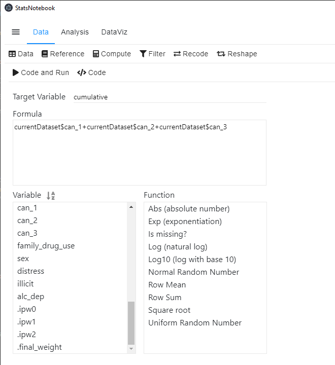
The R code for this operation is simple.

currentDataset$cumulative <- currentDataset$can_1+currentDataset$can_2+currentDataset$can_3

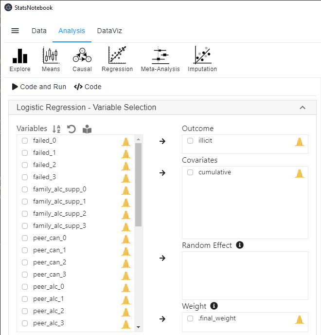
Once we have created the cumulative variable, we can use the survey package to conduct a weighted analysis to estimate the causal effect of cumulative use for cannabis use during adolescence on illicit drug use in young adulthood (age 25). Logistic regression is used because the outcome, illicit drug use, is a dichotomized variable (0: No; 1: Yes).

To conduct a weighted analysis,

1. Click Analysis at the top
2. Click Regression at the top menu
3. Click Logistic regression (linear regression can be used if the outcome is a numeric variable.)
4. In the left panel, select illicit into Outcome, cumulative into Covariate and .final_weight into Weight.

R codes - Weighted analysis

library(survey)

clus <- svydesign(id =~ 1, weights =~ .final_weight, data = currentDataset)
res <- svyglm(illicit ~ cumulative, design = clus,family = binomial)
summary(res)
"Model coefficients and confidence intervals"
cbind(coef(res), confint(res, level = 0.95))

"Odds ratios and confidence intervals"
exp(cbind(OR = coef(res), confint(res, level = 0.95)))


car::infIndexPlot(res)


"Chan, G. and StatsNotebook Team (2020). StatsNotebook. (Version 0.1.0) [Computer Software]. Retrieved from https://www.statsnotebook.io"
"R Core Team (2020). The R Project for Statistical Computing. [Computer software]. Retrieved from https://r-project.org"

The code for a weighted logistic regression is straightforward. The survey package is loaded using the library function. The following line then specifies that the variable .final_weight is used as the weighting variable.

clus <- svydesign(id =~ 1, weights =~ .final_weight, data = currentDataset)

Then we use the following lines to run the weighted logistic regression and request the model results from R.

res <- svyglm(illicit ~ cumulative, design = clus,family = binomial)
summary(res)
"Model coefficients and confidence intervals"
cbind(coef(res), confint(res, level = 0.95))

"Odds ratios and confidence intervals"
exp(cbind(OR = coef(res), confint(res, level = 0.95)))

The codes above produce the following results.

######################################################

Call:
svyglm(formula = illicit ~ cumulative, design = clus, family = binomial)

Survey design:
svydesign(id = ~1, weights = ~.final_weight, data = currentDataset)

Coefficients:
            Estimate Std. Error t value Pr(>|t|)    
(Intercept)  -2.6639     0.2270 -11.734  < 2e-16 ***
cumulative    0.7865     0.2288   3.438 0.000649 ***
---
Signif. codes:  0 '***' 0.001 '**' 0.01 '*' 0.05 '.' 0.1 ' ' 1

(Dispersion parameter for binomial family taken to be 1.000884)

Number of Fisher Scoring iterations: 5


######################################################
[1] "Model coefficients and confidence intervals"

######################################################
                            2.5 %    97.5 %
(Intercept) -2.6639296 -3.1089045 -2.218955
cumulative   0.7865248  0.3380718  1.234978

######################################################
[1] "Odds ratios and confidence intervals"

######################################################
                   OR      2.5 %    97.5 %
(Intercept) 0.0696739 0.04464984 0.1087227
cumulative  2.1957526 1.40224124 3.4383024

######################################################

It should be noted that you may also see the warning message below. This is expected because we have fractional weights.

######################################################
Warning message: non-integer #successes in a binomial glm!

######################################################

Interpretation

Results from the weighted logistic regression indicates that cannabis use was strongly associated with future illicit drug use, b = 0.79, 95% CI = [0.34, 1.23], p < .001. The corresponding odds ratio was 2.20, 95% CI = [1.40, 3.44]. For every additional wave an individual used cannabis, the odds of using illicit drug at age 25 was increased by 2.20 times. It is likely that we can interpret this association as causal, as we have adjusted for key confounding (and time-varying) variables from several important domains such as family, school and peer group. However, it is very likely that the true effect will be slightly smaller due to residual confounding (confounding effect not capture by the variables we used in the analysis.)

Follow our Facebook page or our developer’s Twitter for more tutorials and future updates.