StatsNotebook

Age-period-cohort analysis

29 Mar, 2021 | 12 minutes read

Tags: Analysis, R code, Linear model, Regression

Follow our Facebook page or our developer’s Twitter for more tutorials and future updates.

The tutorial is based on R and StatsNotebook, a graphical interface for R. Visit our Analysis section for other tutorials.

Epidemiologists and social scientists often apply Age-Period-Cohort analysis to disentangle trends of social/health behvaiors into three components.

Age effect - This represents the effect associated with chronological age. For example, young people are more likely to use cannabis for recreational purpose than older people.
Period effect - This represents the effect associated with time period that affects all age groups at the same time. For example, changes in legislation with regards to recreational cannabis use is like to influence behaviors across all age group.
Cohort effect - Epidemiologists and social scientists are often interested in birth cohort, who experienced the same historical and social events at the same age. Cohort effect thus is often used to refered to the variation due to these unique experiences. For example, the baby boomer generation has a higher rate of cannabis use compared to subsequent cohort at the same age.

In this tutorial, we will use a simulalated data based on a nationally representative dataset in Australia and disentangle changes in cannabis use trends into age, period and cohort effect. The challenge of age-period-cohort analysis (APC analysis) has long been identified because the cohort variabls is often directly calcuated from age and period such that

Cohort = Period - Age

In this tutorial, we will use the Hierarchical APC-Corss-Classified Random Effect Model (HACP-CCREM; Yang et al, 2008) to test the age, period and cohort effect on weekly cannabis use. This model is a type of mixed effect model in which the Age effect is entered as a fixed effect and both Cohort and Period are entered as random effects. In this setup, the HACP-CCREM is not different from the typical application of mixed model in which the random effects often represent the contextual effects that influence the outcome. In this case, cohort represents the contextual effect of experiencing the same social and historical context at the same age within the same birth cohort and period effect represents the contextual effect of experiencing the same social and historical context at a certain time period that affects all age group.

Example dataset

In this tutorial, we will use an example dataset simulated based on a national drug survey in Australia.

This data can be loaded using the following code.

library(tidyverse)
currentDataset <- read_csv("https://statsnotebook.io/blog/data_management/example_data/APC_cannabis.csv")

Supposed that the data was collected every three years between 2001 and 2019, there were 7 repeated cross-sectional surveys.

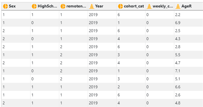
In this dataset, there are 8 variables.

Sex - 1: Male; 2: Female
HighSchool - 0: Not completed high school; 1: completed high school
remoteness - 1: Major cities; 2: Inner regional area; 3: Remote area
Year - Year the data was collected: 2001/2004/2007/2010/2013/2016/2019
cohort_cat - Birth cohort: 1: 1941/50; 2: 1951/60; 3: 1961/70; 4: 1971/80; 5: 1981/90; 6: 1991/2000
weekly_cannabis - Weekly cannabis use: 0: No; 1: Yes
AgeR - Recoded age. The value is calculated by dividing the actual age by 10. This is to facilitate model converence when we add the quadratic term of age into the model.

Age-Period-Cohort model

In this example, we will test the age, period and cohort effect on weekly cannabis use. Since weekly cannabis use is a dichotomized variable (Yes/No), we will firstly fit a mixed effects (multilevel level) logistic model

At level 1, we have

logit P(cannabis_ijk) = b_0jk+b₁Age_ijk+b₂Age²_ijk+b₃Female_ijk+b₄Inner regional_ijk+b₅Remote area_ijk+b₆High School_ijk

where Female, Inner regional, Remote area and High School are indicator variables (i.e. High School = 0 for participants who haven’t finished high school and High School = 1 for participants who finished high school). R will automatically create these indicator variables when a categorical/factor variable is entered into a model. The quadratic term of age is included to capture the potential quadratic effect of age.

At level 2, we have

b_0jk = γ₀+ u_0j + v_0k

where u_0j and v_0k represents the effect of being in period j and birth cohort k, and u_0j ~ N(0, τ_u) and v_0j ~ N(0, τ_v). The u_0j and v_0k have also been referred to as the random effect of period and cohort. It should be noted that the index ijk is the index for individual i in period j and cohort k.

APC analysis in StatsNotebook

In this analysis, after loading the data, we will need to

convert the variable Sex, HighSchool, remoteness, Year, and cohort_cat into factor variables;
centre the age variable at 2 so that the intercept of the model represented the effect of age at 20 years old (i.e. substracting 2 from the age variable); and
create the quadratic term of age, AgeR2.

**See Converting variable type and Converting variable type for a step-by-step guide.

#Converting Sex, HighSchool, Year, cohort_cat and remoteness into factor variable
currentDataset$Sex <- factor(currentDataset$Sex, exclude = c("", NA))
currentDataset$HighSchool <- factor(currentDataset$HighSchool, exclude = c("", NA))
currentDataset$Year <- factor(currentDataset$Year, exclude = c("", NA))
currentDataset$cohort_cat <- factor(currentDataset$cohort_cat, exclude = c("", NA))
currentDataset$remoteness <- factor(currentDataset$remoteness, exclude = c("", NA))

#centre age at 20 years old and create the quadratic term
currentDataset$AgeR = currentDataset$AgeR - 2
currentDataset$AgeR2 = currentDataset$AgeR^2

To fit a Age-Period-Cohort model,

Click Analysis at the top
Click Regression and select Logistic Regression (Binary outcome) from the menu
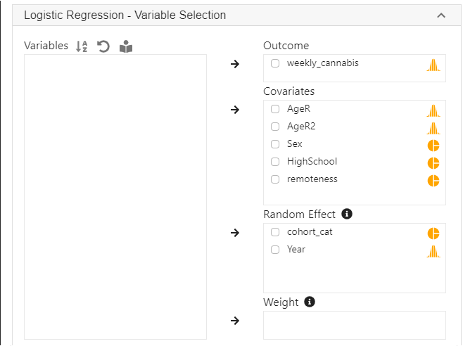
In the left panel, select weekly_cannabis into outcome, AgeR, AgeR2 (the newly created quadratic term of AgeR), Sex, HighSchool and remoteness into Covariates, and select cohort_cat and Year into Random Effect.
Click Code and Run

age-period-cohort analysis instruction 1

library(lme4)

res <- glmer(weekly_cannabis ~ AgeR + AgeR2 + Sex + remoteness + HighSchool + (1 | cohort_cat) + (1 | Year),
  family = binomial,
  data = currentDataset)
summary(res)
confint(res, level = 0.95, method = "Wald")

se <- sqrt(diag(vcov(res)))
z <- -qnorm((1-0.95)/2)
exp(cbind(Est=fixef(res),
  "2.5%"  = fixef(res) - z*se,
  "97.5%" = fixef(res) + z*se))


"Chan, G. and StatsNotebook Team (2020). StatsNotebook. (Version 0.1.1) [Computer Software]. Retrieved from https://www.statsnotebook.io"
"R Core Team (2020). The R Project for Statistical Computing. [Computer software]. Retrieved from https://r-project.org"

R codes explained

The Age-Period-Cohort model in this example is a mixed effects logistic model with random intercepts. The following are from the top section of the generated codes. The analysis uses the glmer function from the lme4 library to fit the model, the summary function to display the model output, and then the confint function to compute the confidence intervals of the parameters using the Wald’s method.

library(lme4)

res <- glmer(weekly_cannabis ~ AgeR + AgeR2 + Sex + remoteness + HighSchool + (1 | cohort_cat) + (1 | Year),
  family = binomial,
  data = currentDataset)
summary(res)
confint(res, level = 0.95, method = "Wald")

The next section of the codes extracts the variance-covariance matrix of the parameters, and calculate the odds ratio and the corresponding confidence intervals of each variable.

se <- sqrt(diag(vcov(res)))
z <- -qnorm((1-0.95)/2)
exp(cbind(Est=fixef(res),
  "2.5%"  = fixef(res) - z*se,
  "97.5%" = fixef(res) + z*se))

The following are excerpt of outputs from the above codes.

Fixed effects:
            Estimate Std. Error z value Pr(>|z|)    
(Intercept) -1.47823    0.19175  -7.709 1.27e-14 ***
AgeR        -0.49014    0.06268  -7.819 5.32e-15 ***
AgeR2        0.01221    0.01186   1.030    0.303    
Sex2        -0.84691    0.03172 -26.697  < 2e-16 ***
remoteness2  0.14050    0.03362   4.179 2.93e-05 ***
remoteness3  0.30242    0.05130   5.895 3.74e-09 ***
HighSchool1 -0.85670    0.03230 -26.521  < 2e-16 ***

The following are odds ratio calculated by exponentiating the model parameters.

                  Est      2.5%     97.5%
(Intercept) 0.2280404 0.1566014 0.3320687
AgeR        0.6125418 0.5417249 0.6926162
AgeR2       1.0122856 0.9890264 1.0360917
Sex2        0.4287377 0.4028924 0.4562409
remoteness2 1.1508512 1.0774569 1.2292450
remoteness3 1.3531320 1.2236971 1.4962576
HighSchool1 0.4245599 0.3985133 0.4523089

As expected, age is strongly associated with reduced odds of using cannabis weekly. The quadratic term of age is not statistically significant and is very close to zero.

In the presence of the quadratic term of age and other variables in the model, to better understand the effect of age on cannabis use, we can use the emmeans package to calculate the probability of weekly cannabis use with the following codes.

library(emmeans)

Age_eff = data.frame()

# Age is centred at 20 years old, and is divided by 10.
# (i.e. 0 means the participant is 20 years old, 1 means 30 years old, etc)
# We use a for loop to calculate the probability of weekly cannabis use 
# when the age "score" is between 0 and 5, with 0.5 increment.
# The calculated probability is stored in a new data frame Age_eff

for (i in 0:10) {
  emm <- emmeans(res,  ~ AgeR + AgeR2,
  at = list(
  AgeR = i/2, AgeR2 = (i/2)^2), type = "response", level = 0.95)
  Age_eff = rbind(data.frame(summary(emm)), Age_eff)
}

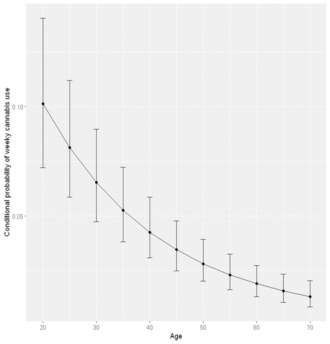
The above codes prodce the following output. This can be considered as the “average” probability averaging across other variables. Note that a score of “0” for age represents 20 years old and a score of “5” represents 70 years old. The column prob is the estimated probability of weekly cannabis use averaged across levels of sex, remoteness, and high school completion.

   AgeR AgeR2       prob          SE  df   asymp.LCL  asymp.UCL
1   5.0 25.00 0.01302441 0.002963280 Inf 0.008329145 0.02031226
2   4.5 20.25 0.01566169 0.003206712 Inf 0.010472891 0.02336060
3   4.0 16.00 0.01893590 0.003566890 Inf 0.013074952 0.02735125
4   3.5 12.25 0.02301558 0.004081239 Inf 0.016237876 0.03252876
5   3.0  9.00 0.02811552 0.004789430 Inf 0.020105526 0.03918906
6   2.5  6.25 0.03450870 0.005735311 Inf 0.024872334 0.04769591
7   2.0  4.00 0.04254035 0.006973858 Inf 0.030786360 0.05851100
8   1.5  2.25 0.05264362 0.008584237 Inf 0.038144305 0.07224044
9   1.0  1.00 0.06535550 0.010690410 Inf 0.047275202 0.08969955
10  0.5  0.25 0.08132988 0.013489649 Inf 0.058509247 0.11199258
11  0.0  0.00 0.10134240 0.017284082 Inf 0.072133577 0.14058661

We can use the ggplot2 library to visualise the age effect using the following codes. See our Data Visualisation guide for tutorials about using ggplot2.

#We transformed back the x axis from "age score" into actual age by adding 2 and then multiplying by 10.
plot <- ggplot(Age_eff, aes(x = ((AgeR+2)*10), y = prob)) +
    geom_point() + 
    geom_line() +
    geom_errorbar(aes(ymin = asymp.LCL, ymax = asymp.UCL), width = 1) +
    xlab("Age") +
    ylab("Probability of weeky cannabis use")
    
plot

Testing the joint cohort and period effect

To test the joint cohort and period effect, we save the current model into a new variable res_cohort_period using the following codes.

res_cohort_period <- res

We then rerun the model without the cohort and period effect (i.e. removing the random effect of cohort and period). This can be done by removing the cohort_cat and year from random effect in StatsNotebook’s menu or by changing the previous codes. The function glm will be used instead of glmer

library(lme4)

res <- glm(weekly_cannabis ~ AgeR + AgeR2 + Sex + remoteness + HighSchool,
  family = binomial,
  data = currentDataset)
summary(res)
confint(res, level = 0.95, method = "Wald")

The above codes can be used to run the analysis without both cohort and period effect. To test the joint cohort and period effect, we can use a likelihood ratio test comparing both models using the anova function.

anova(res_cohort_period, res)

This produces the output below. These results indicate that the model with cohort and period effect fits the data significantly better than the model without, indicating that at least one of the cohort or period effect is significantly different from zero.

Data: currentDataset
Models:
res: weekly_cannabis ~ AgeR + AgeR2 + Sex + remoteness + HighSchool
res_cohort_period: weekly_cannabis ~ AgeR + AgeR2 + Sex + remoteness + HighSchool + 
res_cohort_period:     (1 | cohort_cat) + (1 | Year)
                  npar   AIC   BIC logLik deviance Chisq Df Pr(>Chisq)    
res                  7 34069 34136 -17028    34055                        
res_cohort_period    9 33929 34014 -16956    33911 144.2  2  < 2.2e-16 ***
---
Signif. codes:  0 '***' 0.001 '**' 0.01 '*' 0.05 '.' 0.1 ' ' 1

Testing the cohort effect

We can also test the cohort or period effect individually. For example, we can test the cohort effect by running a model with only period effect, and compare this model with the model with both cohort and period effect. The following is generated by removing cohort_cat from the random effect in StatsNotebook’s menu. We save the model output to the variable res_period instead of the default res.

res <- glmer(weekly_cannabis ~ AgeR + AgeR2 + Sex + remoteness + HighSchool + (1 | Year),
  family = binomial,
  data = currentDataset)
summary(res)
confint(res, level = 0.95, method = "Wald")

#We add the line of codes to save the model result to the variable res_period
res_period <- res

Similarly, we use the anova function to compare the model with both cohort and period effect and the model with only period effect.

anova(res_cohort_period, res_period)

This test produces the following results. The model with both cohort and period effect fits the data significantly better than the model with only period effect. This indicates that the cohort effect is significantly different from zero.

Data: currentDataset
Models:
res_period: weekly_cannabis ~ AgeR + AgeR2 + Sex + remoteness + HighSchool + 
res_period:     (1 | Year)
res_cohort_period: weekly_cannabis ~ AgeR + AgeR2 + Sex + remoteness + HighSchool + 
res_cohort_period:     (1 | cohort_cat) + (1 | Year)
                  npar   AIC   BIC logLik deviance  Chisq Df Pr(>Chisq)    
res_period           8 34049 34125 -17016    34033                         
res_cohort_period    9 33929 34014 -16956    33911 121.81  1  < 2.2e-16 ***
---
Signif. codes:  0 '***' 0.001 '**' 0.01 '*' 0.05 '.' 0.1 ' ' 1

Testing the period effect

The period effect can be tested similiarly by comparing the model with both cohort and period effect against the model with only the cohort effect with the following codes.

library(lme4)

res <- glmer(weekly_cannabis ~ AgeR + AgeR2 + Sex + remoteness + HighSchool + (1 | cohort_cat),
  family = binomial,
  data = currentDataset)
summary(res)
confint(res, level = 0.95, method = "Wald")

res_cohort <- res

anova(res_cohort_period, res_cohort)

These codes produce the following results, which indicates that the period effect is also significantly different from zero.

Data: currentDataset
Models:
res_cohort: weekly_cannabis ~ AgeR + AgeR2 + Sex + remoteness + HighSchool + 
res_cohort:     (1 | cohort_cat)
res_cohort_period: weekly_cannabis ~ AgeR + AgeR2 + Sex + remoteness + HighSchool + 
res_cohort_period:     (1 | cohort_cat) + (1 |cyw195510  Year)
                  npar   AIC   BIC logLik deviance  Chisq Df Pr(>Chisq)    
res_cohort           8 33950 34026 -16967    33934                         
res_cohort_period    9 33929 34014 -16956    33911 23.093  1  1.543e-06 ***
---
Signif. codes:  0 '***' 0.001 '**' 0.01 '*' 0.05 '.' 0.1 ' ' 1

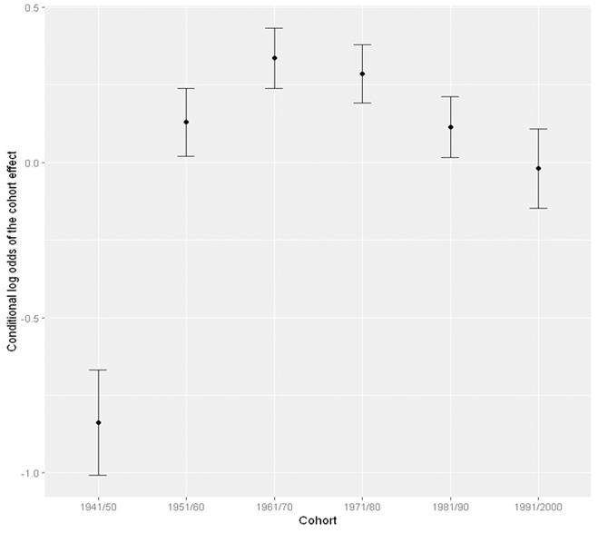
Visualising the cohort effect

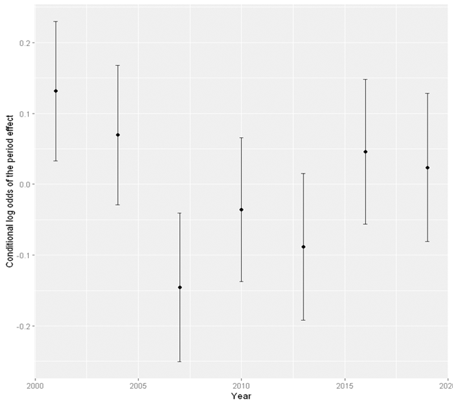
Now that we know there are cohort and period effect on weekly cannabis use. We can visualise both effects. Suppose that we have stored the results from the model with both cohort and period effect into the variable res_cohort_period. We can use the ranef function to extract the random effect components, the cohort and period effect, from this model.

#Extract the random effect
u0 <- ranef(res_cohort_period, condVar = TRUE)
names(u0$Year) <- "est"
names(u0$cohort_cat) <- "est"

#Extract the standard error
period_eff <- data.frame(est = u0$Year, se = sqrt(attr(u0[[1]], "postVar")[1, ,]),
  period = c(2001, 2004, 2007, 2010, 2013, 2016, 2019))
cohort_eff <- data.frame(est = u0$cohort_cat, se = sqrt(attr(u0[[2]], "postVar")[1, ,]),
  cohort = c("1941/50","1951/60","1961/70","1971/80","1981/90","1991/2000"))

period_eff$upper <- period_eff$est + 1.96*period_eff$se
period_eff$lower <- period_eff$est - 1.96*period_eff$se
cohort_eff$upper <- cohort_eff$est + 1.96*cohort_eff$se
cohort_eff$lower <- cohort_eff$est - 1.96*cohort_eff$se

#Visualise the period and cohort effect using ggplot2
plot <- ggplot(period_eff, aes(x = period, y = est)) +
  geom_point() + 
  geom_errorbar(aes(ymin = lower, ymax = upper), width = .2) + 
  xlab("Year") + 
  ylab("Conditional log odds of the period effect")

plot

plot <- ggplot(cohort_eff, aes(x = cohort, y = est)) +
  geom_point() + 
  geom_errorbar(aes(ymin = lower, ymax = upper), width = .2) + 
  xlab("Year") + 
  ylab("Conditional log odds of the cohort effect")

plot

Follow our Facebook page or our developer’s Twitter for more tutorials and future updates.