StatsNotebook
Propensity Score Matching
Tags: Analysis, R code, Propensity score, Causal inference
Follow our Facebook page or our developer’s Twitter for more tutorials and future updates.
The tutorial is based on R and StatsNotebook, a graphical interface for R.
Randomised controlled trials (RCTs) are the gold standard for causal inference. In RCTs, randomisation removes all confoundings between the treatment (exposure) and control group. However, RCTs are not always feasible due to ethical or logistic issues (e.g., testing the causal impact of smoking on lung cancer). Propensity score matching can be used to emulate the balance between treatment and control group in an observational study. At its simplest, propensity score matching matches each individual in the treatment group to an individual in the control group based on their propensity score. For each individual, the propensity score can be intuitively considered as the probability of recentiving treatment, calcuated from a range of covariates (and potential confounders). Two individuals, one from treatment and one from control group, is considered to be a match if the difference between their propensity score is small. Unmatched participants are discarded.
After matching, the treatment group and the control group should have very similar characteristics. A simple regression model can be used to estimate the treatment effect on the outcome. Cluster-robust standard errors are required for correct inference.
Example research questions
- Is smoking associated with psychological distress?
In this setup, the treatment variable is smoking; the outcome variable is psychological distress. This research question will be addressed by propensity score matching. We will first match each smoker in the dataset to a non-smoker based on a range of covariates, including sex (male/ female), indigenous status (indigenous or not), education level (high school completion), marital status (partnered or not), region of residence (major cities, inner regional or outer regional), language background (English speaking or not), age and risky alcohol use (Yes/ No).
Propensity score matching analysis involves two steps.
- Match each smoker to a non-smoker based on propensity score, which is calculated based on a range of covariates.
- Check if balance between smokers (treatment/exposure group) and non-smokers (control group) is achieved (i.e., both groups having similar characteristics). If balance is achieved, a simple regression analysis with cluster-robust standard error can be used to estimate the effect of smoking on psychological distress.
We will first show the R code for this analysis below, and we will provide a step-by-step guide on how to complete this analysis. We use the Psychological distress and smoking dataset, which can be loaded using the following codes (internet connection is required)
library(tidyverse)
currentDataset <- read_csv("https://raw.githubusercontent.com/gckc123/ExampleData/main/smoking_psyc_distress.csv")
There are ten variables in this dataset.
- Sex (0: Female; 1: Male)
- indigenous - Ingigenous status (0: Non-indigenous; 1: indigenous)
- high_school - Education level (0: not finished high school; 1: finished high school)
- partnered - Marital status (0: not partnered; 1: partnered)
- remoteness - region of residence (0: major cities; 1: inner regional; 2: outer regional)
- language - Language background (0: non-English speaking; 1: English speaking)
- Smoker - Smoking status (0: non-smoker; 1: smoker)
- risky_alcohol - Risky alcohol use (0: not risky; 1: risky)
- psyc_distress - Psychological distress. Measure ranges from 10 to 50.
- age - Age of the participants
R codes for matching (Step 1)
The following is the compete codes for our propensity score matching example.
#Since remoteness is a categorical variable with more than two categories. It is necessary to convert
#it into a factor variable.
#For other categorical variable with only 2 levels, this is optional if the variable is coded as 0 and 1.
currentDataset$remoteness <- factor(currentDataset$remoteness, exclude = c("", NA))

#The MatchIt, lmtest and sandwich libraries are used.
library(MatchIt)
library(lmtest)
library(sandwich)

#Using the mathcit function from MatchIt to match each smoker with a non-smoker (1 to 1 matching) based on
#sex, indigeneity status, high school completion, marital status (partnered or not),
#region of residence (major cities, inner regional, outer regional), language background (English speaking Yes/No)
#and risky alcohol drinking (Yes/No)
match_obj <- matchit(smoker ~ sex + indigeneity + high_school + partnered + remoteness + language + risky_alcohol + age,
  data = currentDataset, method = "nearest", distance ="glm",
  ratio = 1,
  replace = FALSE)
summary(match_obj)

#plotting the balance between smokers and non-smokers
plot(match_obj, type = "jitter", interactive = FALSE)
plot(summary(match_obj), abs = FALSE)
Using StatsNotebook for matching (Step 1)
Prior to running the propensity score matching, it is always a good practice to visualise the data and conduct a descriptive analysis.
To conduct propensity score matching,
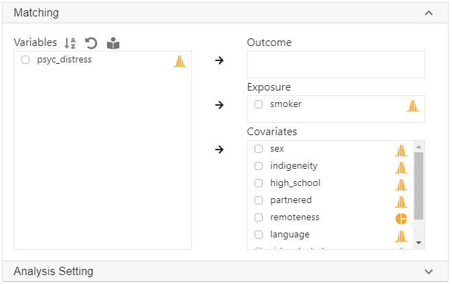
- Click Analysis at the top;
- Click Causal and select Matching from the menu
- In the left panel, select smoker into Exposure, and select sex, indigeneity, high_school, partnered, remoteness, lauguage psyc_distress and age into Covariates.
- remoteness is a categorical variable with three levels (major cities, inner regional and outer regional). If it is not yet coded as factor, we will need to manually convert it into a factor variable.
- sex, indigeneity, high_school, partnered and language are also categorical variable. But since they are binary (i.e., only have two levels coded as 0 and 1), it is not necessary to convert them into factor variable.
- Click Code and Run at top. The above R code will be generated in a block on the right panel and the results will be presented below the R codes.

R codes explained - Matching
The following is a key section of the generated codes.
match_obj <- matchit(smoker ~ sex + indigeneity + high_school + partnered + remoteness + language + risky_alcohol + age,
  data = currentDataset, method = "nearest", distance ="glm",
  ratio = 1,
  replace = FALSE)
summary(match_obj)
This code tells R to run a propensity score matching using the matchit function from the MatchIt library. The left side of the “~” symbol specifies the exposure variable; the right side specifies the covariates. The results from this propensity score matching is then printed out using the summary function.
- The distance parameter specifies that generalised linear model is used to calculate the propensity score based on all covariates (distance = “glm”); Other models such as generalised boosted model (gbm) or generalized additive model (gam) can be used.
- The method parameter specifies that matching is based on nearest matching (method = “nearest”); Other methods such as “optimal” and “exact” can be used.
- The ratio parameter specifies that one to one matching is used (ratio = 1). A higher ratio will increase the number of samples from the control group that will be included. Therefore, less observations will be discarded. However a higher matching ratio by definition will produce worse matches.
- The replace parameter specifies that the matching is conducted without replacement.
These settings generally produce satisfactory results and will be sufficient in many scenarios.
This code produces the result summary below.
######################################################

Call:
matchit(formula = smoker ~ sex + indigeneity + high_school +
    partnered + remoteness + language + risky_alcohol + age,
    data = currentDataset, method = "nearest", distance = "glm",
    replace = FALSE, ratio = 1)

Summary of Balance for All Data:
              Means Treated Means Control Std. Mean Diff. Var. Ratio eCDF Mean
distance             0.1852        0.1130          0.6304     2.0778    0.2033
sex                  0.4938        0.4421          0.1035          .    0.0518
indigeneity          0.0524        0.0175          0.1565          .    0.0349
high_school          0.4220        0.6378         -0.4370          .    0.2158
partnered            0.4630        0.6913         -0.4578          .    0.2283
remoteness0          0.5852        0.6773         -0.1870          .    0.0921
remoteness1          0.2177        0.1900          0.0670          .    0.0277
remoteness2          0.1971        0.1327          0.1621          .    0.0645
language             0.9579        0.9130          0.2234          .    0.0449
risky_alcohol        0.6427        0.5411          0.2120          .    0.1016
age                 51.6057       53.7824         -0.1676     0.8214    0.0441
              eCDF Max
distance        0.3185
sex             0.0518
indigeneity     0.0349
high_school     0.2158
partnered       0.2283
remoteness0     0.0921
remoteness1     0.0277
remoteness2     0.0645
language        0.0449
risky_alcohol   0.1016
age             0.1020


Summary of Balance for Matched Data:
              Means Treated Means Control Std. Mean Diff. Var. Ratio eCDF Mean
distance             0.1852        0.1847          0.0042     1.0209    0.0002
sex                  0.4938        0.5010         -0.0144          .    0.0072
indigeneity          0.0524        0.0370          0.0691          .    0.0154
high_school          0.4220        0.4107          0.0229          .    0.0113
partnered            0.4630        0.4764         -0.0268          .    0.0133
remoteness0          0.5852        0.5986         -0.0271          .    0.0133
remoteness1          0.2177        0.2146          0.0075          .    0.0031
remoteness2          0.1971        0.1869          0.0258          .    0.0103
language             0.9579        0.9620         -0.0205          .    0.0041
risky_alcohol        0.6427        0.6407          0.0043          .    0.0021
age                 51.6057       51.2064          0.0307     0.9171    0.0150
              eCDF Max Std. Pair Dist.
distance        0.0113          0.0052
sex             0.0072          0.2854
indigeneity     0.0154          0.2627
high_school     0.0113          0.1725
partnered       0.0133          0.1874
remoteness0     0.0133          0.3230
remoteness1     0.0031          0.2463
remoteness2     0.0103          0.3407
language        0.0041          0.1329
risky_alcohol   0.0021          0.2957
age             0.0390          0.3717

Percent Balance Improvement:
              Std. Mean Diff. Var. Ratio eCDF Mean eCDF Max
distance                 99.3       97.2      99.9     96.5
sex                      86.1          .      86.1     86.1
indigeneity              55.8          .      55.8     55.8
high_school              94.8          .      94.8     94.8
partnered                94.2          .      94.2     94.2
remoteness0              85.5          .      85.5     85.5
remoteness1              88.9          .      88.9     88.9
remoteness2              84.1          .      84.1     84.1
language                 90.8          .      90.8     90.8
risky_alcohol            98.0          .      98.0     98.0
age                      81.7       56.0      66.0     61.8

Sample Sizes:
          Control Treated
All          7026     974
Matched       974     974
Unmatched    6052       0
Discarded       0       0

######################################################
Matching results explained
In the top section of the results, the balance between smoker and non-smoker group in each of the covariates are shown. The column on Std. Mean Diff. shows that there are substantial difference in nearly all covariates between smokers and non-smokers (a standardised mean difference great than 0.1 can be considered as substantial difference).
In the middle section, the balance between smoker and non-smoker group after matching are shown. The standardised mean differences are now all close to zero for all covariates, indicating that a good balance is achieved.
The last section shows that there are 7026 non-smokers and 974 smokers in the original sample. All smokers are matched to a corresponding non-smokers. The remaining 6052 non-smokers are not matched to any smokers and can be discarded in subsequent analysis. Applied researchers sometimes are concerned about discarding a large number of unmatched participants. However, this is usually not an issue if all treated participants are matched, and good balance is archived.
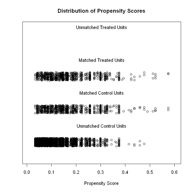
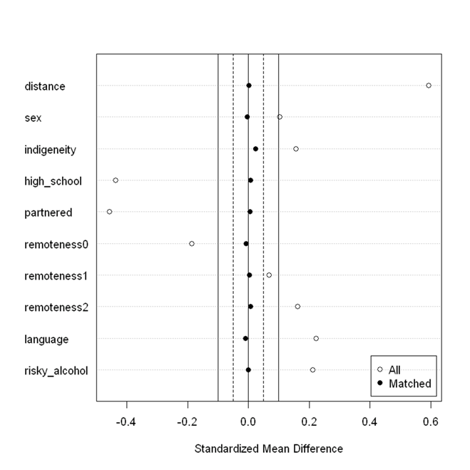
The above codes also produce the following two figures. The first one visualises the distribution of propensity score in the matched treated group, matched control group and the unmatched control group. Propensity score matching will not be appropriate if there is not a satisfactory overlap in the propensity score distribution between the matched treated group and the matched untreated group. The second figure visualises the balance in propensity score and all covariates before and after matching. Similar to the results from the table, there are substantial difference in all covariates between smokers and non-smokers before matching, but the difference is close to zero after matching, indicating a very good balance.


R codes for outcome analysis (Step 2)
Once we achieve a good balance between the treatment and control group after matching, we can proceed to the next step to analyse the difference in outcome between the two groups. We can analyse the data as if the data are from an RCT using a regression analysis. However, for correct inference, cluster-robust standard error is needed.
#Extract the matched data and save the data into the variable matched_data
matched_data <- match.data(match_obj)

#Run regression model with psychological distress as the outcome, and smoker as the only predictor
#We need to specify the weights - Matched participants have a weight of 1, unmatched participants
res <- lm(psyc_distress ~ smoker, data = matched_data, weights = weights)

#Test the coefficient using cluster robust standard error
coeftest(res, vcov. = vcovCL, cluster = ~subclass)
#Calculate the confidence intervals based on cluster robust standard error
coefci(res, vcov. = vcovCL, cluster = ~subclass, level = 0.95)
Using StatsNotebook for outcome analysis (Step 2)
The following steps will generate the R codes for both matching and outcome analysis. It should be noted that we should only conduct outcome analysis after we achieve a satisfactory balance between treatment and control group.
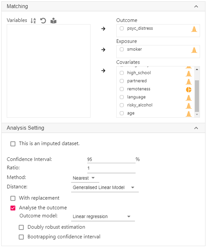
- In addition to the procedure in step 1, we now select psyc_distress into Outcome
- Expand the Analysis setting panel in the bottom, click Analyse the outcome.
- Click Code and Run at top. This will generate both the codes for propensity score matching and outcome analysis.

R output and interpretation
The followings are the output from the outcome analysis. The results indicate that psychological distress among smokers is 1.66 point higher than non-smokers (95% CI [1.08, 2.24]).
######################################################

t test of coefficients:

            Estimate Std. Error t value  Pr(>|t|)
(Intercept) 15.65298    0.20093  77.904 < 2.2e-16 ***
smoker       1.66016    0.29657   5.598 2.477e-08 ***
---
Signif. codes:  0 '***' 0.001 '**' 0.01 '*' 0.05 '.' 0.1 ' ' 1


######################################################
                2.5 %    97.5 %
(Intercept) 15.258922 16.047032
smoker       1.078545  2.241783

######################################################
Write-up
Propensity score matching was used to estimate the effect of smoking on psychological distress. The propensity score were estimated using logistic regression based on sex, indigenous status, education level (completed high school or not), marital status (partnered or not), region of residence (major cities, inner regional or outer regional), language background (English speaking Yes/No), risky alcohol use (Yes/ No) and age. One-to-one nearest neighbour matching was used. All smokers (N = 974) were matched to a non-smoker. Good balance was achieved between the smoker and non-smoker group, with all standardized mean differences below 0.1 after matching.
To estimate the effect of smoking on psychological distress, a linear regression with psychological distress as the outcome and smoking status (smoker/ non-smoker) as the exposure was fitted. Cluster-robust variance was used to estimate the standard error. It is estimated that smoking increases psychological distress by 1.66 point (95% CI [1.08, 2.24], p < .001>).
All analyses were conducted in StatsNotebook (Chan and StatsNotebook team, 2020) using R 4.1 and the MatchIt package (Stuart, King, Imai and Ho, 2011).
Citation
Chan, G. and StatsNotebook Team (2020). StatsNotebook. [Computer Software]. Retrieved from https://www.statsnotebook.io
Stuart, King, Imai and Ho. (2011). MatchIt: nonparametric preprocessing for parametric causal inference. Journal of statistical software.
Follow our Facebook page or our developer’s Twitter for more tutorials and future updates.