StatsNotebook

The tutorial is based on R and StatsNotebook, a graphical interface for R.

Outliers and violations of distributional assumptions are common in many area of research. These issues might introduce substantial bias in the analysis and potentially lead to grossly incorrect inferences. Traditionally, outliers are identified through manual inspection of the data; violations of normality are often addressed by data transformation. Other forms of assumption violations, such as heterogeneity in variance, can be more challenging to address (Assumptions for linear regression can be checked using residual plots). Robust regression is a technique that can reduce the impact of outliers, violation of the distribution assumption and heterogeneity in variance. It should be noted that the linearity assumption is still needed for proper inference using robust regression.

In this example, we will use the Stars dataset from the Robustbase package. We have built this example data into StatsNotebook and it can be loaded using the instructions provided here.

This dataset can also be loaded using the following codes

library(tidyverse)
currentDataset <- read_csv("https://statsnotebook.io/blog/data_management/example_data/stars.csv")

In this dataset, there are two variables.

1. temperature represents the surface temperature of a star
2. light represents the light intensity of a star

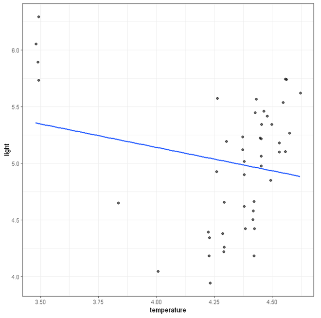
The figure below shows the scatterplot between temperature and light with a regression line. At first glance, there appears to be a downward trend. However, this trend may only be caused by the few outliers at the top left corner.

We will now demonstrate the use of robust regression to adjust for these outliers.

Using StatsNotebook

Steps for running a Robust regression in StatsNotebook are nearly the same as running a linear regression.

1. Click Analysis at the top;
2. Click Regression and select Linear Regression (Numeric outcome) from the menu
3. In the left panel, select light into Outcome, and select temperature into Covariates.
4. Expand the Analysis setting panel, and click Robust regression

R codes explained

The codes for a robust regression are nearly the same as those for linear regression, except that we use the lmrob function from the robustbase package instead of the lm function for linear regression.

library(robustbase) 
res <- lmrob(light ~ temperature,
  data=currentDataset)
summary(res)
cbind(coef(res),confint(res, level = 0.95))


"Chan, G. and StatsNotebook Team (2020). StatsNotebook. (Version 0.1.0) [Computer Software]. Retrieved from https://www.statsnotebook.io"
"R Core Team (2020). The R Project for Statistical Computing. [Computer software]. Retrieved from https://r-project.org"

Interpretation

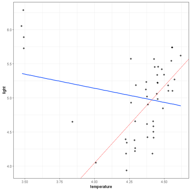
The output from robust regression is also very similar to those from linear regression. The only exception now is that that the observations are now weighted based on how deviant they are, and also robust standard errors will be computed for model estimates. After adjusting for a few outliers, we find that temperature is positively associated with light intensity, b = 2.25, 95% CI (0.70, 3.80), p =.005. We also show the regression line estimated from the robust regression in the figure below. The blue line is the regression line from ordinary linear regression and the red one is the regression line from the robust regression.

Call:
lmrob(formula = light ~ temperature, data = currentDataset)
 \--> method = "MM"
Residuals:
     Min       1Q   Median       3Q      Max 
-0.80959 -0.28838  0.00282  0.36668  3.39585 

Coefficients:
            Estimate Std. Error t value Pr(>|t|)   
(Intercept)  -4.9694     3.4100  -1.457  0.15198   
temperature   2.2532     0.7691   2.930  0.00531 **
---
Signif. codes:  0 '***' 0.001 '**' 0.01 '*' 0.05 '.' 0.1 ' ' 1

Robust residual standard error: 0.4715 
Multiple R-squared:  0.3737,	Adjusted R-squared:  0.3598 
Convergence in 15 IRWLS iterations

Robustness weights: 
 4 observations c(11,20,30,34) are outliers with |weight| = 0 ( < 0.0021); 
 4 weights are ~= 1. The remaining 39 ones are summarized as
   Min. 1st Qu.  Median    Mean 3rd Qu.    Max. 
 0.6533  0.9171  0.9593  0.9318  0.9848  0.9986 
Algorithmic parameters: 
       tuning.chi                bb        tuning.psi        refine.tol 
        1.548e+00         5.000e-01         4.685e+00         1.000e-07 
          rel.tol         scale.tol         solve.tol       eps.outlier 
        1.000e-07         1.000e-10         1.000e-07         2.128e-03 
            eps.x warn.limit.reject warn.limit.meanrw 
        8.404e-12         5.000e-01         5.000e-01 
     nResample         max.it       best.r.s       k.fast.s          k.max 
           500             50              2              1            200 
   maxit.scale      trace.lev            mts     compute.rd fast.s.large.n 
           200              0           1000              0           2000 
                  psi           subsampling                   cov 
           "bisquare"         "nonsingular"         ".vcov.avar1" 
compute.outlier.stats 
                 "SM" 
seed : int(0) 

######################################################
                            2.5 %   97.5 %
(Intercept) -4.969388 -11.8375510 1.898775
temperature  2.253161   0.7041936 3.802129

Follow our Facebook page or our developer’s Twitter for more tutorials and future updates.