StatsNotebook

Linear Regression

18 Sep, 2020 | 10 minutes read

Follow our Facebook page or our developer’s Twitter for more tutorials and future updates.

The tutorial is based on R and StatsNotebook, a graphical interface for R.

Linear regression is a technique for examining the relationship between a dependent variable (outcome) and a set of independent variables (predictors). This tutorial demonstrates how to conduct a linear regression in StatsNotebook using the following example. We will also provide an example write-up in APA style.

Example research questions

Are the Big 5 personality traits, Agreeableness, Conscientiousness, Extraversion, Neuroticism, and Openness, associated with depression?
Is sex associated with depression? (i.e. Are there sex differences in depression?)

In this setup, the dependent variable is depression; the independent variables are Agreeableness, Conscientiousness, Extraversion, Neuroticism, Openness and sex. The above two research questions will be addressed by linear regression.

We will first show the R code for this analysis below, and we will provide a step-by-step guide on how to complete this analysis. We use the Personality, which can be loaded using the following codes

library(tidyverse)
currentDataset <- read_csv("https://statsnotebook.io/blog/data_management/example_data/personality.csv")

R codes

The following is the compete codes for our linear regression and multiple imputation example.

"Linear regression"
res <- lm(Depression ~ Agreeableness + Conscientiousness + Extraversion + Neuroticism + Openness + Sex,
  data=currentDataset)
summary(res)
cbind(coef(res), confint(res, level = 0.95))

library(car)

res.std <- rstandard(res)
plot(res.std, ylab="Standardized Residuals")

"Outlier Test. Observations with a Bonferroni p < .01 might be considered as outliers and might need further investigation."
outlierTest(res)
infIndexPlot(res)

"Residual plots, curvature tests and normality plot"
residualPlots(res)
ggplot(as.data.frame(res.std), aes(sample = res.std)) +
  geom_qq() +
  geom_qq_line()

"Variance inflation factor (VIF >=5 indicates high level of multicollinearity)"
vif(res)


"Chan, G. and StatsNotebook Team (2020). StatsNotebook. (Version 0.1.0) [Computer Software]. Retrieved from https://www.statsnotebook.io"
"R Core Team (2020). The R Project for Statistical Computing. [Computer software]. Retrieved from https://r-project.org"

Using StatsNotebook

Prior to running the linear regression analysis, it is always a good practice to visualise the data and conduct a descriptive analysis.

To run a linear regression,

Click Analysis at the top;
Click Regression and select Linear Regression (Numeric outcome) from the menu
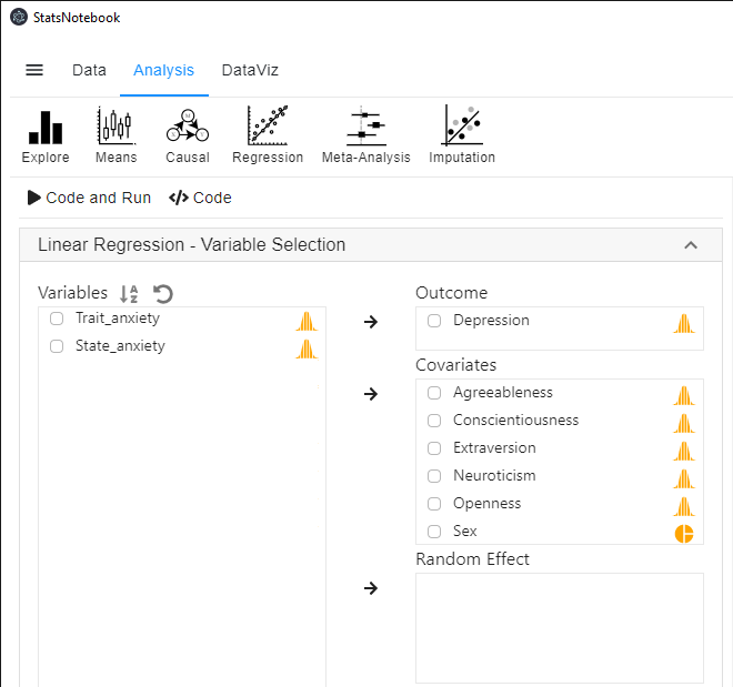
In the left panel, select Depression into Outcome, and select Agreeableness, Conscientiousness, Extraversion, Neuroticism, Openness and Sex into Covariates.
- Sex is a categorical variable. If it is not yet coded as factor, we will need to manually convert it into a factor variable.
- Female is chosen as the reference level for sex by default. To change the reference level, see setting reference level for categorical variable for step-by-step guide..
Click Code and Run at top. The above R code will be generated in a block on the right panel and the results will be presented below the R codes.

R codes explained - Regression analysis

The following is from the top section of the generated codes.

res <- lm(Depression ~ Agreeableness + Conscientiousness + Extraversion + Neuroticism + Openness + Sex,
  data=currentDataset)
summary(res)
cbind(coef(res), confint(res, level = 0.95))

This code tells R to run a linear regression using the lm function. The left side of the “~” symbol specifies the dependent variable; the right side specifies the independent variables. The results from this regression analysis is then printed out using the summary function. Lastly, the cbind, coef and confint functions are used to print the model coefficients with the corresponding 95% confidence intervals.

This code produces the model summary below.

######################################################

Call:
lm(formula = Depression ~ Agreeableness + Conscientiousness + 
    Extraversion + Neuroticism + Openness + Sex, data = currentDataset)

Residuals:
     Min       1Q   Median       3Q      Max 
-10.3954  -3.5621  -0.5515   2.1011  18.2826 

Coefficients:
                  Estimate Std. Error t value Pr(>|t|)    
(Intercept)        7.98352    3.57490   2.233   0.0270 *  
Agreeableness     -0.01498    0.02859  -0.524   0.6011    
Conscientiousness -0.01702    0.02231  -0.763   0.4467    
Extraversion      -0.02104    0.01839  -1.144   0.2546    
Neuroticism        0.14296    0.01891   7.559 3.94e-12 ***
Openness          -0.05455    0.02454  -2.222   0.0278 *  
SexMale           -0.87264    0.88739  -0.983   0.3270    
---
Signif. codes:  0 '***' 0.001 '**' 0.01 '*' 0.05 '.' 0.1 ' ' 1

Residual standard error: 5.091 on 148 degrees of freedom
  (76 observations deleted due to missingness)
Multiple R-squared:  0.3319,	Adjusted R-squared:  0.3048 
F-statistic: 12.26 on 6 and 148 DF,  p-value: 3.608e-11


######################################################
                                    2.5 %       97.5 %
(Intercept)        7.98352411  0.91909104 15.047957174
Agreeableness     -0.01497977 -0.07148527  0.041525721
Conscientiousness -0.01701989 -0.06110049  0.027060703
Extraversion      -0.02103749 -0.05738767  0.015312701
Neuroticism        0.14295833  0.10558358  0.180333083
Openness          -0.05454570 -0.10304908 -0.006042319
SexMale           -0.87264011 -2.62623258  0.880952360

######################################################

Interpretation

The R-sq indicates that the model explains 33.19% of the variance in depression. It should be noted that 76 observations have missing data and thus have been removed from the analysis. See Regression with missing data for a more appropriate way to handle the missing data in this analysis.

Residual standard error: 5.091 on 148 degrees of freedom
  (76 observations deleted due to missingness)
Multiple R-squared:  0.3319,	Adjusted R-squared:  0.3048 
F-statistic: 12.26 on 6 and 148 DF,  p-value: 3.608e-11

The model coefficients are shown in the section below.

The p-value provides an indication of the level of evidence against a null effect (i.e. zero association) for each of the variables. Traditionally, a p-value under 0.05 represents a statistically significant finding. It should be noted that there is debate on how the p-value should be used, and conclusion should not be drawn solely on the reliance on on the p-value.

There is evidence that a higher level of neuroticism is associated with a higher level of depression. The coefficient of neuroticism is 0.14, indicating that one unit increase in neuroticism is associated with 0.14 unit decrease in depression. The result also shows that a higher level of openness is associated with a lower level of depression. The coefficient of openness is -0.05, indicating that a one unit increase in openness is associated with 0.05 unit decrease in depression. The other three traits, agreeableness, conscientiousness and extraversion are not significantly associated with depression. The estimated coefficients are very close to zero.

Using a significance level of 0.05, we conclude that openness and neuroticism are significantly associated with depression, but agreeableness, conscientiousness and extraversion are not. Depression for males on average is 0.87 unit lower than females, but the effect is not statistically significant.

Coefficients:
                  Estimate Std. Error t value Pr(>|t|)    
(Intercept)        7.98352    3.57490   2.233   0.0270 *  
Agreeableness     -0.01498    0.02859  -0.524   0.6011    
Conscientiousness -0.01702    0.02231  -0.763   0.4467    
Extraversion      -0.02104    0.01839  -1.144   0.2546    
Neuroticism        0.14296    0.01891   7.559 3.94e-12 ***
Openness          -0.05455    0.02454  -2.222   0.0278 *  
SexMale           -0.87264    0.88739  -0.983   0.3270    
---
Signif. codes:  0 '***' 0.001 '**' 0.01 '*' 0.05 '.' 0.1 ' ' 1

Emphasis should be placed on the 95% confidence interval of these coefficients because statistical significance provides no information about the effect size. From this analysis, we are 95% confident that the effect of neuroticism on depression is between 0.11 and 0.18. The 95% confidence interval for openness is (-0.103, -0.006). Thus the effect of openness could be close to zero because one end of the confidence interval (the upper end in this case) is very close to zero.

                                    2.5 %       97.5 %
(Intercept)        7.98352411  0.91909104 15.047957174
Agreeableness     -0.01497977 -0.07148527  0.041525721
Conscientiousness -0.01701989 -0.06110049  0.027060703
Extraversion      -0.02103749 -0.05738767  0.015312701
Neuroticism        0.14295833  0.10558358  0.180333083
Openness          -0.05454570 -0.10304908 -0.006042319
SexMale           -0.87264011 -2.62623258  0.880952360

R codes explained - Model diagnostic

To evaluate the validity of the above results, we will need to check if the assumptions of linear regression are satisfied. There are four key assumptions of linear regression.

Linearity
Homoscedasticity (constant variance of the residuals)
Normality (residuals are normally distributed)
Independence of observations

The independence assumption can be ensured if the sample is a random sample. When there is dependency in the data, other statistical methods, such as Linear mixed model, can be used.

In addition, we also need to check for multicollinearity, outliers and/or influential observations (i.e. observations that may have a large impact on the model coefficients).

To check the other three assumptions (i.e. Linearity, homoscedasticity and normality) and perform model diagnostic, we will need to use several functions from the car library. To load this library, we use the following code.

library(car)

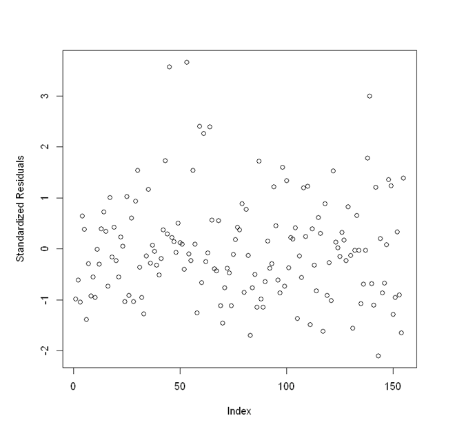
The following two lines of codes are used to generate a residual plot.

res.std <- rstandard(res)
plot(res.std, ylab="Standardized Residuals")

All the points should be randomly scattered around 0, with approximately 95% of the points falling between -2 and 2 standardized residuals. Points with a large standardized residual may be outliers.

The following lines of codes allow us to examine if there are outliers and if there are any observations that might have a large influence on the model estimates.

"Outlier Test. Observations with a Bonferroni p < .01 might be considered as outliers and might need further investigation."
outlierTest(res)
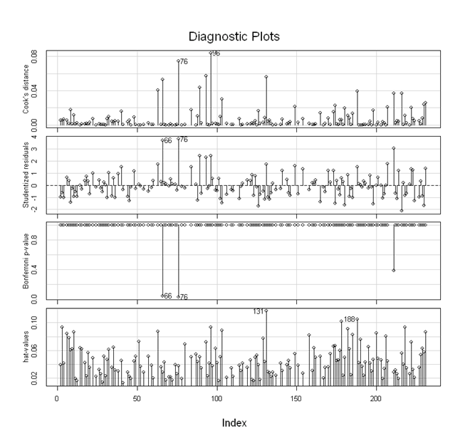
infIndexPlot(res)

This code first produces results from an outlier test. While there is no clear guideline on the cut-off, observations with a Bonferroni corrected p-value < .01 may need further investigation. For example, these observations will need to be checked for errors. Researchers can also perform sensitivity analyses by removing the outliers and comparing the results from the full analysis with their inclusion.

######################################################
[1] "Outlier Test. Observations with a Bonferroni p < .01 might be considered as outliers and might need further investigation."

######################################################
   rstudent unadjusted p-value Bonferroni p
76 3.824964         0.00019277     0.029879
66 3.722572         0.00028023     0.043436

######################################################

The following plot is produced by the infIndexPlot function. We can focus on the top panel on Cook’s distance. Observations with a Cook’s distance close to 1 indicates a high impact on the model coefficients. There is no influence observation in this analysis despite the existence of two observations with large residuals.

The following code is used to produce more diagnostic plots and a normality plot.

"Residual plots, curvature tests and normality plot"
residualPlots(res)
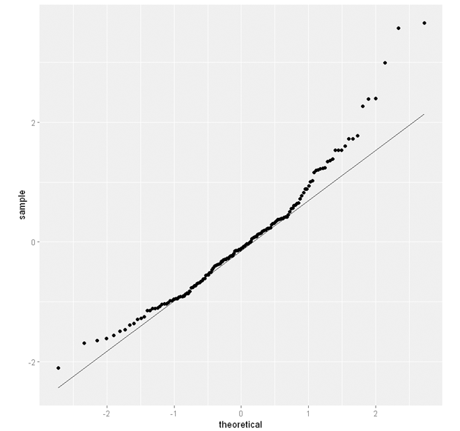
ggplot(as.data.frame(res.std), aes(sample = res.std)) +
  geom_qq() +
  geom_qq_line()

Below is a set of diagnostic plots.

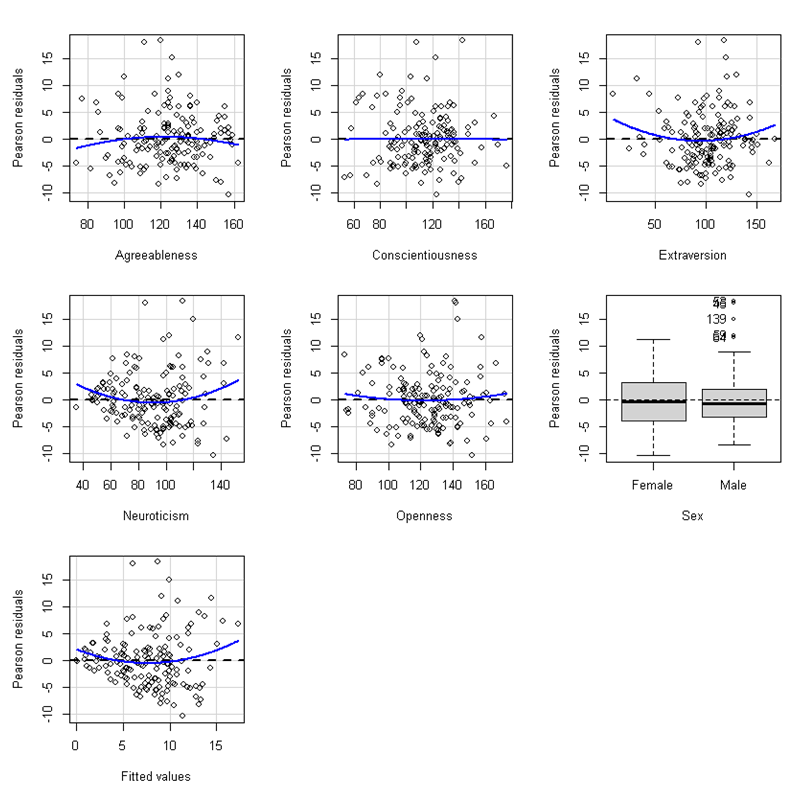
The residuals are plotted against each of the independent variables and the fitted values. Ideally, points on these plots need to be randomly scattered around 0. Any non-linear pattern (e.g. curvature) in the residual plots indicate that the linearity assumption is violated. A fanning in or fanning out pattern indicates the homoscedasticity assumption is violated. See Residual plots and assumption checking for examples of plots that demonstrate a violation of the linearity assumption and the homoscedasticity assumption.

The following are the results from curvature tests for each of the variables. A quadratic term is added to each of the plots and a curvature test tests if the quadratic term is zero. A test with a p-value < .01 may indicate the presence of a non-linear trend (U-shape or inverted U-shape).

                  Test stat Pr(>|Test stat|)  
Agreeableness       -1.0679          0.28730  
Conscientiousness   -0.0964          0.92332  
Extraversion         1.5893          0.11414  
Neuroticism          1.8781          0.06235 .
Openness             0.7340          0.46410  
Sex                                           
Tukey test           1.7834          0.07452 .
---
Signif. codes:  0 '***' 0.001 '**' 0.01 '*' 0.05 '.' 0.1 ' ' 1

Below is a normality plot. If the residual is normally distributed, the points need to follow a straight line. In this case, there is evidence that the normality assumption is violated. When the normality assumption is violated, we can try a log-transformation of the dependent variable or use other analytic methods such as robust regression to evaluate whether the violation has a substantial impact on the model estimates.

Lastly, the following codes compute the Variance Inflation Factor (VIF).

"Variance inflation factor (VIF >=5 indicates high level of multicollinearity)"
vif(res)

A VIF over 5 indicates a high level of multicollinearity. In this analysis, multicollinearity is not a concern as all the VIFs are small.

    Agreeableness Conscientiousness      Extraversion       Neuroticism 
         1.726463          1.467871          1.466692          1.176284 
         Openness               Sex 
         1.535307          1.117182

Example write-up (APA style)

Table 1. Results from linear regression.

Variables	b	95% CI	p
Agreeableness	-0.01	(-0.07, 0.04)	0.601
Conscientiousness	-0.02	(-0.06, 0.03)	0.447
Extraversion	-0.02	(-0.06, 0.01)	0.255
Neuroticism	0.14	(0.11, 0.18)	< .001
Openness	-0.05	(-0.10, -0.01)	.028
Sex (Ref: Female)
Male	-0.87	(-2.62, 0.88)	0.327

Linear regression is used to examine the association between depression and agreeableness, conscientiousness, extraversion, neuroticism, openness and sex. Results are shown in Table 1. Using a significance level of 0.05, results indicate that higher neuroticism (b = 0.14, 95% CI [0.11, 0.18], p < .001) and lower openness (b = -0.05, 95% CI [-0.10, -0.01], p = .028) are associated with depression. Other variables were not significantly associated with depression, and their effects are close to zero. Overall, the model explains 33.19% of the variance in depression. Analyses were conducted in StatsNotebook (Chan and StatsNotebook Team, 2020) with R (R Core Team, 2020).

Citation

Chan, G. and StatsNotebook Team (2020). StatsNotebook. [Computer Software]. Retrieved from https://www.statsnotebook.io
Chan, G (2020). Linear regression. Retrieved from https://www.statsnotebook.io/blog/analysis/regression/

Follow our Facebook page or our developer’s Twitter for more tutorials and future updates.