StatsNotebook
Linear regression with missing data
Tags: Analysis, R code, Regression, Missing data
Follow our Facebook page or our developer’s Twitter for more tutorials and future updates.
The tutorial is based on R and StatsNotebook, a graphical interface for R.
In many area of research, missing data is a norm rather than an exception. Dropping observations/ participants with missing data is usually not appropriate as it reduces statistical power and also may introduce bias in analysis. This tutorial will demonstrate a simple way in StatsNotebook to handle missing data using multiple imputation.
In our linear regression tutorial, we use the personality dataset to examine two research qeustions.
- Are the Big 5 personality traits, Agreeableness, Conscientiousness, Extraversion, Neuroticism, and Openness, associated with depression?
- Is sex associated with depression?
In our original analysis, participants with missing data in any of the analysis variables are excluded. The initial sample size is 231. After excluding participants with missing data, the sample size reduces to 155 - a reduction of 33%.
Multiple imputation is a widely used method to handle missing data. This can generally increase power and reduce bias due to missingness. StatsNotebook provides a simple interface to incorporate multiple imputation into linear regression analysis.
This tutorial builds on our tutorial on linear regression, and re-examine the above two research questions using multiple imputation and linear regression. We firstly show the R codes for this analysis, and will provide a step-by-step guide on how to complete this analysis. We use the Personality dataset in this example, which can be loaded into using the following codes.
library(tidyverse)
currentDataset <- read_csv("https://statsnotebook.io/blog/data_management/example_data/personality.csv")
Two variables, .imp and .id will be added to the dataset on successful imputation. The .imp is the imputation number, and zero indicates the original dataset. The .id is a unique identifier for each observation in the dataset.
R codes
The following is the compete codes for our linear regression example.
"Impute missing data"
library(mice)

formulas <- make.formulas(currentDataset)

formulas$Agreeableness =Agreeableness ~ Conscientiousness + Extraversion + Neuroticism + Openness + Sex + Depression
formulas$Conscientiousness =Conscientiousness ~ Agreeableness + Extraversion + Neuroticism + Openness + Sex + Depression
formulas$Extraversion =Extraversion ~ Agreeableness + Conscientiousness + Neuroticism + Openness + Sex + Depression
formulas$Neuroticism =Neuroticism ~ Agreeableness + Conscientiousness + Extraversion + Openness + Sex + Depression
formulas$Openness =Openness ~ Agreeableness + Conscientiousness + Extraversion + Neuroticism + Sex + Depression
formulas$Sex =Sex ~ Agreeableness + Conscientiousness + Extraversion + Neuroticism + Openness + Depression
formulas$Depression =Depression ~ Agreeableness + Conscientiousness + Extraversion + Neuroticism + Openness + Sex

meth <- make.method(currentDataset)
meth["Trait_anxiety"] <- ""
meth["State_anxiety"] <- ""

imputedDataset <- parlmice(currentDataset,
  method = meth,
  formulas = formulas,
  m = 35,
  n.core = 15,
  n.imp.core = 3)

plot(imputedDataset)
currentDataset <- complete(imputedDataset, action = "long", include = TRUE)

"Linear regression"
res <- with(imputedDataset,
  lm(Depression ~ Agreeableness + Conscientiousness + Extraversion + Neuroticism + Openness + Sex))
summary(pool(res), conf.int = TRUE, conf.level = 0.95)

res1 <- res$analyses[[1]]
library(car)

res.std <- rstandard(res1)
plot(res.std, ylab="Standardized Residuals")

"Outlier Test. Observations with a Bonferroni p < .05 might be considered as outliers and might need further investigation."
outlierTest(res1)
infIndexPlot(res1)

"Residual plots, curvature tests and normality plot"
residualPlots(res1)
ggplot(as.data.frame(res.std), aes(sample = res.std)) +
  geom_qq() +
  geom_qq_line()

"Variance inflation factor (VIF >=5 indicates high level of multicollinearity)"
vif(res1)


"Chan, G. and StatsNotebook Team (2020). StatsNotebook. (Version 0.1.0) [Computer Software]. Retrieved from https://www.statsnotebook.io"
"R Core Team (2020). The R Project for Statistical Computing. [Computer software]. Retrieved from https://r-project.org"
Using StatsNotebook
Prior to running the linear regression analysis, it is always a good practice to visualise the data and conduct descriptive analysis.
To conduct multiple imputation and linear regression analysis,
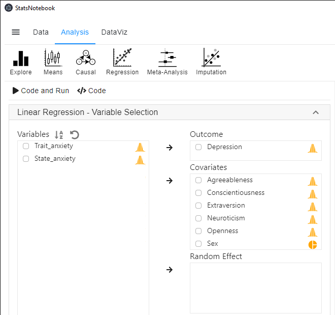
- Click Analysis at the top;
- Click Regression and select Linear Regression (Numberic outcome) from the menu
- In the left panel, select Depression into Outcome, and select Agreeableness, Conscientiousness, Extraversion, Neuroticism, Openness and Sex into Covariates.
- Sex is a categorical variable. If it is not yet coded as factor, we will need to manually convert it into a factor variable.

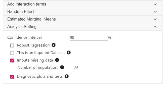
- On the left panel, scroll down and expand the Analysis setting panel. Check Impute missing data and enter the number of imputation required. In this example, we request 35 imputations.
- As a rule of thumb, the number of imputation should be close to the percentage of observations with missing data.

R codes explained - Multiple imputation
The following is from the top section of the generated codes.
library(mice)

formulas <- make.formulas(currentDataset)

formulas$Agreeableness =Agreeableness ~ Conscientiousness + Extraversion + Neuroticism + Openness + Sex + Depression
formulas$Conscientiousness =Conscientiousness ~ Agreeableness + Extraversion + Neuroticism + Openness + Sex + Depression
formulas$Extraversion =Extraversion ~ Agreeableness + Conscientiousness + Neuroticism + Openness + Sex + Depression
formulas$Neuroticism =Neuroticism ~ Agreeableness + Conscientiousness + Extraversion + Openness + Sex + Depression
formulas$Openness =Openness ~ Agreeableness + Conscientiousness + Extraversion + Neuroticism + Sex + Depression
formulas$Sex =Sex ~ Agreeableness + Conscientiousness + Extraversion + Neuroticism + Openness + Depression
formulas$Depression =Depression ~ Agreeableness + Conscientiousness + Extraversion + Neuroticism + Openness + Sex

meth <- make.method(currentDataset)
meth["Trait_anxiety"] <- ""
meth["State_anxiety"] <- ""

imputedDataset <- parlmice(currentDataset,
  method = meth,
  formulas = formulas,
  m = 35,
  n.core = 15,
  n.imp.core = 3)

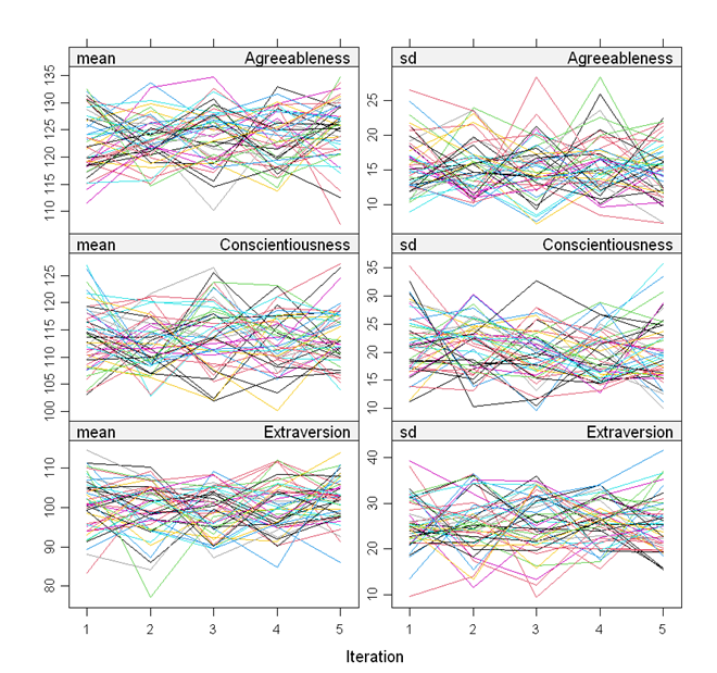
plot(imputedDataset)
currentDataset <- complete(imputedDataset, action = "long", include = TRUE)
We use the mice library in R to perform multiple imputation. The above codes firstly specifies how each variables are imputed. Only variables used in the regression analysis will be used for imputation. To include additional variables in the imputation, see the multiple imputation.
The only visible output is a set of diagnostic plot. The lines in all plots should be freely intermingled. Non-convergence will be indicated by clearly separated lines.

The following codes are then used to conduct linear regression using the imputed datasets.
"Linear regression"
res <- with(imputedDataset,
  lm(Depression ~ Agreeableness + Conscientiousness + Extraversion + Neuroticism + Openness + Sex))
summary(pool(res), conf.int = TRUE, conf.level = 0.95)
Below is the output from this analysis.
               term     estimate  std.error   statistic       df      p.value
1       (Intercept)  7.715447666 3.12663997  2.46764825 174.0538 1.456720e-02
2     Agreeableness -0.001189368 0.02497579 -0.04762083 158.8576 9.620782e-01
3 Conscientiousness -0.018990634 0.01964996 -0.96644620 130.7906 3.356046e-01
4      Extraversion -0.013549340 0.01559403 -0.86887995 176.7667 3.860910e-01
5       Neuroticism  0.128537235 0.01657551  7.75464787 165.6124 8.557599e-13
6          Openness -0.060743216 0.02205921 -2.75364405 134.9948 6.705879e-03
7           SexMale -1.227802866 0.76103616 -1.61333051 195.1378 1.082887e-01
        2.5 %      97.5 %
1  1.54443849 13.88645685
2 -0.05051680  0.04813806
3 -0.05786353  0.01988226
4 -0.04432377  0.01722509
5  0.09581069  0.16126378
6 -0.10436956 -0.01711687
7 -2.72871486  0.27310912
Interpretation
In this example, the coefficients of the 5 personality traits from the analysis using imputation are similar to those from complete data analysis. However, it should be noted that the p-value of openness is now much smaller, indicating that the evidence for the association between openness and depression was stronger (despite the effect size being similar). This is due to increase power from multiple imputation.
Example Write-up
Table 1. Results from linear regression.
| Variables | b | 95% CI | p |
|---|---|---|---|
| Agreeableness | -0.00 | (-0.05, 0.05) | 0.962 |
| Conscientiousness | -0.02 | (-0.02, 0.02) | 0.336 |
| Extraversion | -0.01 | (-0.04, 0.02) | 0.386 |
| Neuroticism | 0.13 | (0.10, 0.16) | < .001 |
| Openness | -0.06 | (-0.10, -0.02) | .007 |
| Sex (Ref: Female) | |||
| Male | -1.23 | (-2.73, 0.27) | 0.108 |
The intial sample consists of 231 participants. Seventy six participants (33%) have missing data in at least one of the analysis variable. Thirty-five datasets were imputed using multiple imputation to fill in the missing values (Rubin, 2009). Linear regression is used to examine the association between depression and agreeableness, conscientiousness, extraversion, neuroticism, openness and sex. Results are shown in Table 1. Using a significance level of 0.05, results indicate that higher neuroticism (b = 0.13, 95% CI [0.09, 0.16], p < .001) and lower openness (b = -0.06, 95% CI [-0.10, -0.02], p = .007) are associated with depression. Other variables are not significantly associated with depression, and their effects are close to zero. Analyses are conducted in StatsNotebook (Chan and StatsNotebook Team, 2020) with R (R Core Team, 2020)
Model diagnostic
At the moment, model diagnostic is only based on the first imputed dataset. The interpretation for the model diagnostic is thus the same as those for analysis based on complete data analysis.
Citation
Chan, G. and StatsNotebook Team (2020). StatsNotebook. [Computer Software]. Retrieved from https://www.statsnotebook.io
Chan, G (2020). Linear regression with missing data. Retrieved from https://www.statsnotebook.io/blog/analysis/regression_missingdata/
R Core Team (2020). The R Project for Statistical Computing. [Computer software]. Retrieved from https://r-project.org
Rubin, D. B. (2009). Multiple imputation for nonresponse in surveys. New York, John Wiley & Sons.
Follow our Facebook page or our developer’s Twitter for more tutorials and future updates.